Research logs - PhD day-to-day log
Jun 23, 17:40 - Tornike
Overview
Currently, I’m actively searching for possible PhD topics - in ML. I almost feel like a journeyman, having some knowledge, but not enough to prove my worth as an expert within the field.
The one topic that got me interested today is the so called binary neural networks - NNs that rely on “cheaper” binary operations (XOR, OR, AND, etc.) in order to simulate the capabilities of MatMul-powered networks. There is an interesting paper on that topic, with title “XNOR-Net: ImageNet Classification Using Binary Convolutional Neural Networks”.
In this paper, authors approximate the Conv operation in two different ways - both relying on binary ops.
Brief (and probably bad) overview of XNOR-Networks paper
In the first case, which is aptly called Binary-Weights-Network, the inputs \(I\) are still usual fp32 [BN, C, W, H] matrices. However, the Conv operation \(I * W\), where \(W\) is the kernel, is decomposed into \(I * W \approx ( I \oplus B ) * \alpha\), where \(B\) is a constrained binary kernel \(B \in \{ -1, +1 \} ^ {C \times W \times H}\) and \(\alpha\) is a mean of \(W\), and so \(\alpha \in R^{+}\).
The benefits of this approach are as follows:
- \(B\) can theoretically be stored in a 32-times smaller space.
- The \(\oplus\) can be performed using just additions and subtractions.
The second case, the titular XNOR-Network, also binarizes the inputs.The approximation looks like this:
Where \(\otimes\) is the binary convolution (same as above, can be done without multiplications), the \(\odot\) is elementwise dot product, and the \(K\alpha\), serves the same purpose as the \(\alpha\) in the Binary-Weights-Network - to contain the scaling factors (And I arguably didn’t spend enough time to understand this fully).
The inputs are binarized just as you’d expect - just a plain \(sign(\cdot)\) of the inputs is enough to get the job done. The authors then derive the appropriate gradients for these operations and use a SGD with momentum to train the network.
Authors note that a speedup can only be gained from using this architecture when the CPU of the machine can’t “fuse the multiplication and addition as a single cycle operation… On those CPUs, Binary-Weight-Networks does not deliver speed up”.
At this point, I began searching for related code for this paper - found this github repo, and played with it for a little bit on kaggle, and then… lost interest. Why:
- I didn’t think that this CNN weights compression approach is going to be useful in the foreseeable future. Yes, it does reduce size requirements, but currently, the trend is to make larger models, not smaller ones. The average consumer hardware capabilities are also increasing. If you don’t believe me, take a look at the average consumer-facing software size in GB, year after year. It’s increasing, getting less and less efficient (the trend even has a name - “bloatware”), while also getting more popular. Because hardware allows this. There is no need (yet) to make something more complex in order to save space. Which leads me to another point…
- Things are already pretty damn hard in ML :) Unless someone has a really good reason to save those extra bytes, the effort fixing the bugs that the extra complexity would bring wouldn’t be worth it. Not to mention that a lot of the ideas and tools already developed for non-binary networks might not work with the binary networks without some adjustments.
Conclusion
Binary networks allows for up to 32x storage size reduction for Convnets and up to 64x times inference speedup for older CPU architectures. It does this by approximating Conv operation with binary operations and scaling. Both inference and training modes are available and discussed within the paper. While initially interested, I reasoned that the architecture wouldn’t be popular because hardware improvements incentivise less efficient but simpler approaches in ML.
Jun 29, 17:40 - Tornike
Overview
Not having TPUs buried in my backyard (and also not having a backyard either), I considered exploring the current deep learnng for tabular data research. Also, Kaggle is hosting a a monthly “Tabular Playground” competitions, which also got me interested. Current challenge (expires in 2 days), is about data imputation (guessing missing values). And it kind of feels like a generalized tabular prediction task - instead of a single target column, you have many. It’s almost like an industrial version of sudoku.
Either way, the research into a new topic starts with a good literature review, which forms a bird’s eye view of the topic. I chose an excellent paper “Deep Neural Networks and Tabular Data: A Survey”, by Vadim Borisov et al., first published in 2021/10.
Contents of Deep Neural Networks and Tabular Data: A Survey
The abstract neatly rounds up what the following papers discuss - there are three families of models for tabular DNN, and that tree-based learners still outperform DNN approaches by a sizeable margin - especially in supervised settings.
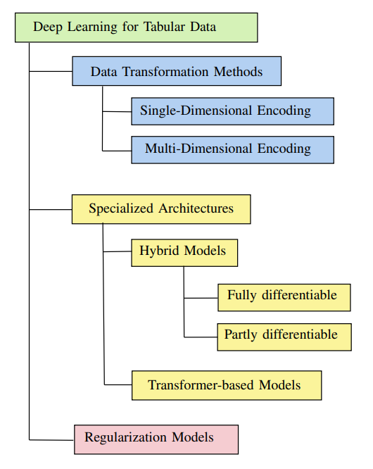
Paper introduces three main classes of models in tabular DNNs.
Data transformation methods are focused on transforming the tabular data in a way that better enables DNNs to learn. This includes the good ol’ fashioned categorical encoding schemes, such as one-hot encoding, hashing, target encoding, and others. Other approaches are mostly encoder-decoder style models that learn the mapping \(x \approx \hat{f}(x,W)\). These models can be also divided within single dimensional and multi dimensional groups, with the former transforming features independently and the latter mapping entire record to optimized representation.
Specialized architectures are divided into hybrid fully differentiable and partially differentiable classes and transformer based models. Hybrid models are, in essence, an attempt to merge DNNs with GBDTs. Only the fully differentiable ones provide a way to SGD-optimize the entire pipeline. Transformer models avoid merging with GDBTs and instead rely on attention to complex representations.
Regularization models attempt to find optimal regularization approaches to combat higher complexity of the DNNs, which they claim is the main reason as to why the DNNs aren’t able to generalize well on tabular data.
Further, the main issues that hinder tabular DNN performance are listed as follows:
- Data quality is usually much worse, with many missing values, outliers, numerical errors (man-made or otherwise), and size of data. Frequent class imbalance is also a frequent problem. Whereas, most modern tree-based learners can handle missing, extreme and different values by design.
- Correlations are complex or non-existent. No spatial, token-wise correlations - think of the success Convnets achieved, with their inductive bias. The convnet is ready to capture the most important visual characteristics from the image, by design. This is possible because there is a strong spatial correlation between pixels in real-world images. In tabular data, these relationships have to be learned from scratch.
- Preprocessing is vital for tabular DNN methods, complicating the data-to-prediction pipeline and requiring extra computation, whereas tree-based learners like CatBoost can handle categorical values internally. Main approaches to feature encoding are later discussed in the paper.
- Model sensitivity to all features of the sample. For image data, a shift in the target usually means a lot of pixels changing their values at once. Whereas in tabular data, just a single feature could decide the value of the target. Tree-based learners handle these cases well by making a decision based on a single feature and a threshold, whereas DNNs (particularly dense FFNs) weigh each feature value with equal weight - diluting the most important signal with what is essentially noise.
Models (Just the ones I found personally interesting)
TODO
Jun 30, 14:20 - Tornike
Working on applying transformers for tabular data. An interesting idea I have yet to test out is that we replace continuous variables with categoricals. To make that work, we will need to reduce the number of unique continuous values. That can be done in two ways (still have to test which is best):
- Standard scale everything
- Then round to 3-4 significant digits (depending on comp. resources)
- Every different value is a different category This comes with an issue: If a segment of values is empty, no category will be created such that it maps to that segment. Thus, the network won’t be able to output that value at all.
- Standard scale everything
- Get a \(N\) as high as comp. resources allow. Select a region of \(R = \pm M\sigma\), where \(M\) is manually selected.
- Divide region \(R\) into \(N\) segments. Assign each segment a unique embedding.
- Values that fall into that segment, get assigned the same embedding.
- Add several additional categories for NaNs, infs and possibly outliers (if someone wants to manually label outliers).
Jul 4, 18:25 - Tornike
Just launched the first long-running notebook. Didn’t yet to add validation eval, but the model is being saved, so I’ll just validate from the saved model. I’m using the 'hf-internal-testing/tiny-random-distilbert' model - with random weights. I noticed several possible sources of bugs in the future:
- It’s possible that random embeddings aren’t scaled properly (this pytorch tutorial uniform randomly inits weights in the range of \(\pm0.1\)).
- The current approach I’m testing is to assign each unique rounded float value a unique embedding. However, there’s a question of whether or not same value from two different columns can share an embedding. I think it’s going to be infeasible to do so. To allow model to differentiate between values of different columns, I re-enable positional encoding (default is off in tinydisilbert config). Hopefully this works. Otherwise, I’d need to encode column info some other way.
- Set
max_position_embeddingsto 80 - i.e. the number of columns. Inputs are never going to be larger than this, so this is a good optimization. - Just found out that by default the
lossfunction ignoreslabelswhich equal -100. i.e. If \(y^{i}_{target} = -100\) then \(\mathcal{L}(x^{i}_{pred}, y^{i}_{target}) = 0\). So model doesn’t wrongfully learn to produce tokens that correspond to theNaNvalue. - Speaking of
NaNvalues and other special tokens, once current run is done, I’m going to add a few extra tokens to embedding space (might have to set up manual mapping from float to cat). Currently I’m thinking of assigning embeddings to $N$ segments of \(\pm 3\sigma\) range + 5 extra segments for NaN, \(+\infty\), \(-\infty\), \(o^{-}_{outlier}\), \(o^{+}_{outlier}\), where extreme values are values above and below of the \(\pm 3\sigma\).
Jul 8, 22:44 - Tornike
I’ve heard that transformers are quite compute-hungry - they are one of the most general (least biased) model out there (next to GNNs) and require much more training than, say, CNNs that have built-in aptitude to capture pixel-data. Now - I have experienced that fact firsthand. It took the tinybert 1 hour to achieve just 20% val accuracy. Next time I’m going to change a few things:
- Instead use an even smaller encoder (something like 4 embed-dim + 2 attn heads and single layer?)
- Also plot training loss (I expect it to overfit quite rapidly, with increasing model size)
- Maybe try tinybert on even smaller datasets - fitting a line in 2d and observing how predictions change with increasing complexity.

Jul 15, 22:35 - Tornike
Four words: “Well regularized Simple Nets”. This is the name of the a 2021 paper that proposes a novel approach to tabular deep learning. I believe the importance of effective learning from tabular data needs no introduction - it is the most abundant and most general form of data out there. The paper attempts to dethrone the wildly popular XGBoost and other GBDT frameworks by using simple MLPs (9 layers, 512 neurons, activation selu, classification task). We know that this set-up doesn’t compare to XGBoost’s performance, however, the authors actually manage to beat XGBoost and various other architectures on most datasets (see below figure, “MLP-C” is the proposed approach).
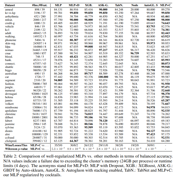
The authors achieve this impressive feat by creating a “cocktail” of regularization techniques (dropout, weight decay, augmentation, etc.) and finding the best combination for the fixed network, using the validation set (20% of labelled data), using bayesian optimization. The best combination is then applied to the model, and is trained on train + validation data anew. The above figure shows test-set results.